
We support you in precise parameter identification using a simplified upstream process for the production of a recombinant bioproduct as an example. Our goal is to capture the essential dynamics of your genetically modified organism in a mathematical bioprocess model. The resulting tailored model then forms a robust basis for strategic decisions: you can perform in‑depth process analyses such as sensitivity studies or systematically optimise your bioprocess to substantially increase yield.
(Status: June 2022)
Application example
The genetically modified organism \(\color{#4daf4a}{X}\) (cf. E. coli) is cultivated in an ideally mixed stirred‑tank reactor. Formation of the recombinant product \(\color{#377eb8}{P}\) is induced by adding an activator \(a\) (cf. IPTG) at time \(t_{\text{a}}\).[1] Biomass growth and product formation compete for the same substrate \(\color{#ff7f00}{S}\) (cf. glucose). At the end of the process time \(t_{\text{harvest}}\), the product is harvested and processed.
It is known that high substrate concentrations \(\color{#ff7f00}{S}\) inhibit biomass growth; after activator addition, most substrate is consumed for product formation. Increasing product concentration further inhibits biomass growth, product formation ceases once the substrate is depleted, and biomass decay can be observed.
Parameter identification requires a sufficiently rich experimental dataset and a suitable bioprocess model. The data must capture all essential system properties, so multiple experiments must be conducted to generate measurement data. In these experiments, selected control variables are systematically varied. In this example, the initial biomass concentration \(X_0\), initial substrate concentration \(S_0\), activation time \(t_{\text{a}}\) and harvest time \(t_{\text{harvest}}\) are treated as control variables.
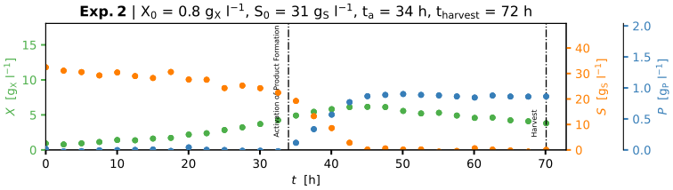
Using design of experiments together with appropriate control‑variable settings, relevant experiments can be planned and executed. Here, the dataset consists of 9 experiments, as visualised in the figure below (click to enlarge):
The underlying bioprocess model is given by the following system of differential equations:[2][3]
\[ \dot{X} = \mu(S,P)\,X - k_{\text{d}} X \] \[ \dot{S} = -\frac{\mu(S,P)\,X}{Y_{\text{X,S}}} -\frac{\rho(S,a)\,X}{Y_{\text{P,S}}} - m X \] \[ \dot{P} = \rho(S,a)\,X \]Here, \(k_{\text{d}}\) and \(m\) denote constant rates for biomass decay and substrate consumption for cellular maintenance, respectively. The yield coefficients \(Y_{\text{X,S}}\) and \(Y_{\text{P,S}}\) represent the ratios of consumed substrate to newly formed biomass and product. Biomass growth/decay and product formation are described by the kinetic functions:[2]
\[ \mu(S,P) = \frac{\mu_{\max} S} {K_{\text{S}} + S + \frac{S^2}{K_{\text{I,S}}} + \frac{S P}{K_{\text{I,P}}}} \] \[ \rho(S,a) = \begin{cases} 0, & a = 0 \\[4pt] \dfrac{\rho_{\max} S}{K_{\text{P}} + S}, & a = 1 \end{cases} \]Methodological background
Parameter identification – estimation of all model parameter values – is formulated as a mathematical minimisation problem. The goal is to find parameter values that minimise the deviation between experimental data and simulated trajectories. A range of established methods exist for this task; here, a least‑squares objective is combined with a direct heuristic search method (downhill simplex).[4]
It is assumed that all parameters are structurally and practically identifiable.[5] The following diagram illustrates the identification workflow and its components:
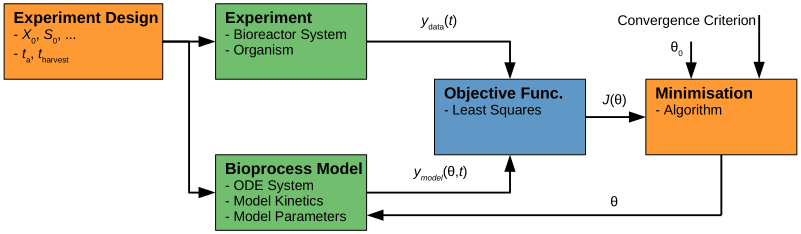
To run parameter identification, parameter bounds and initial values \(\theta_0\) must be specified for the parameter vector \(\theta\). In most applications, bounds can be constrained using prior knowledge and basic kinetic or mathematical considerations. The table below lists the model parameters and their bounds used in this example:
| Symbol | Description | Bounds | Unit | |
|---|---|---|---|---|
| lower | upper | |||
| $\mu_{\max}$ | maximum specific growth rate | $0.1$ | $0.7$ | $\text{h}^{-1}$ |
| $\rho_{\max}$ | maximum specific product formation rate | $0.01$ | $0.05$ | $\text{h}^{-1}$ |
| $K_{\text{S}}$ | substrate half‑saturation constant | $0.5$ | $5$ | $\text{g}_{\text{S}} \cdot \text{L}^{-1}$ |
| $K_{\text{P}}$ | product half‑saturation constant | $0.5$ | $5$ | $\text{g}_{\text{S}} \cdot \text{L}^{-1}$ |
| $K_{\text{I,S}}$ | substrate inhibition constant | $5$ | $50$ | $\text{g}_{\text{S}} \cdot \text{L}^{-1}$ |
| $K_{\text{I,P}}$ | product inhibition constant | $0.05$ | $2$ | $\text{g}_{\text{P}} \cdot \text{L}^{-1}$ |
| $k_{\text{d}}$ | specific biomass decay rate | $0$ | $0.1$ | $\text{h}^{-1}$ |
| $m$ | specific substrate maintenance rate | $0$ | $0.1$ | $\text{g}_{\text{S}} \cdot \text{g}_{\text{X}}^{-1} \cdot \text{h}^{-1}$ |
| $Y_{\text{X,S}}$ | yield coefficient biomass/substrate | $0.1$ | $1$ | $\text{g}_{\text{X}} \cdot \text{g}_{\text{S}}^{-1}$ |
| $Y_{\text{P,S}}$ | yield coefficient product/substrate | $0.01$ | $0.1$ | $\text{g}_{\text{P}} \cdot \text{g}_{\text{S}}^{-1}$ |
Choosing suitable starting values is often challenging. Ideally, they come from prior knowledge or can be inferred empirically for very simple models. For dynamic, nonlinear models with many parameters, as in this example, suitable initial vectors \(\theta_0\) are generated using methods such as full‑factorial combinations or stochastic/probabilistic sampling strategies (e.g. Sobol, Saltelli) within the parameter bounds.[6–8]
Optimal parameter values \(\Omega\) are obtained by minimising the objective function \(J(\theta)\):
\[ \Omega = \underset{\theta}{\mathrm{argmin}}\bigl(J(\theta)\bigr) \] \[ J(\theta) = \sum_{j=1}^{k} \sum_{i=1}^{n} \left( y_{\text{data}}(t_{j,i}) - y_{\text{model}}(\theta, t_{j,i}) \right)^2 \]This objective sums the squared differences between the observed data \(y_{\text{data}}(t_{j,i})\) and the simulated model output \(y_{\text{model}}(\theta, t_{j,i})\). Indices \(i = 1,\ldots,n\) and \(j = 1,\ldots,k\) refer to the sampling time within each time series and to the experiment index, respectively.
Results
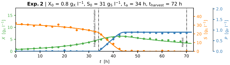
In this example, 106 initial parameter combinations were generated within the bounds using the Saltelli sampling scheme, and each was evaluated via the objective \(J(\theta)\).[8] Subsequent minimisation from promising starts converged to the parameter set shown below:
| Symbol | Description | Value | Unit |
|---|---|---|---|
| $\mu_{\max}$ | maximum specific growth rate | $0.32$ | $\text{h}^{-1}$ |
| $\rho_{\max}$ | maximum specific product formation rate | $0.020$ | $\text{h}^{-1}$ |
| $K_{\text{S}}$ | substrate half‑saturation constant | $2.3$ | $\text{g}_{\text{S}} \cdot \text{L}^{-1}$ |
| $K_{\text{P}}$ | product half‑saturation constant | $1.6$ | $\text{g}_{\text{S}} \cdot \text{L}^{-1}$ |
| $K_{\text{I,S}}$ | substrate inhibition constant | $9.1$ | $\text{g}_{\text{S}} \cdot \text{L}^{-1}$ |
| $K_{\text{I,P}}$ | product inhibition constant | $0.10$ | $\text{g}_{\text{P}} \cdot \text{L}^{-1}$ |
| $k_{\text{d}}$ | specific biomass decay rate | $0.024$ | $\text{h}^{-1}$ |
| $m$ | specific substrate maintenance rate | $0.034$ | $\text{g}_{\text{S}} \cdot \text{g}_{\text{X}}^{-1} \cdot \text{h}^{-1}$ |
| $Y_{\text{X,S}}$ | yield biomass/substrate | $0.60$ | $\text{g}_{\text{X}} \cdot \text{g}_{\text{S}}^{-1}$ |
| $Y_{\text{P,S}}$ | yield product/substrate | $0.053$ | $\text{g}_{\text{P}} \cdot \text{g}_{\text{S}}^{-1}$ |
The figure below shows that the calibrated model reproduces all essential system properties observed in the experiments (click to enlarge):
The calibrated bioprocess model can subsequently be used for further analysis (e.g. sensitivity analysis) or process optimisation (e.g. yield maximisation).
References
- [1] L. Gao, Y. Ren, Y. Ma, J. Lin and J. Lin: Modeling and simulation of production of metallothionein and red fluorescent fusion protein by recombinant Escherichia coli using graphical programming. In: Modeling, Programming and Simulations Using LabVIEW Software, IntechOpen, London, 2011. doi: 10.5772/14091
- [2] D. Voet and J. G. Voet: Biochemistry. New York: John Wiley & Sons, 1990. ISBN: 0-471-61769-5
- [3] A. Kremling: Grundlagen der mathematischen Modellierung. In: Kompendium Systembiologie, Vieweg+Teubner, 2012. doi: 10.1007/978-3-8348-8607-1_3
- [4] J. A. Nelder and R. Mead: A simplex method for function minimization. In: The Computer Journal, 7(4):308–313, 1965. doi: 10.1093/comjnl/7.4.308
- [5] A. Raue et al.: Structural and practical identifiability analysis of partially observed dynamical models by exploiting the profile likelihood. In: Bioinformatics, 25(15):1923–1929, 2009. doi: 10.1093/bioinformatics/btp358
- [6] B. Tang: Orthogonal array-based latin hypercubes. In: J. Am. Stat. Assoc., 88(424):1392–1397, 1993. doi: 10.2307/2291282
- [7] I. M. Sobol: Distribution of points in a cube and approximate evaluation of integrals. In: Zh. Vych. Mat. Mat. Fiz., 7:784–802, 1967.
- [8] A. Saltelli: Making best use of model evaluations to compute sensitivity indices. In: Computer Physics Communications, 145:280–297, 2002. doi: 10.1016/S0010-4655(02)00280-1