Infection models and their simulation

With mathematical infection modelling, we make the complex dynamics of disease spread transparent and predictable for you. We translate biological factors and social interactions into precise agent-based simulations or classical differential equation models. By digitally computing influencing factors such as infection rates, latency periods and contact densities, we simulate realistic scenarios and future infection peaks. This provides a solid, data-driven basis for anticipating epidemiological risks and digitally validating intervention measures.

(Status: April 2021)

Background

The spread of a disease depends on its biological properties, on the contacts between individuals in different groups of a population and on individual or combined probabilities, which in reality may be influenced by a variety of factors (e.g. contact duration, immune status, type of contact such as touch or body fluids, and many more). In the following, the term “infection model” refers to the dynamics of a disease without directly modelling the interaction between pathogen and host organism.

In mathematical epidemiology, one option for modelling this process is to treat all contacts between individuals as single events governed by specific rules, or to explicitly model each individual. Agent-based modelling (ABM) offers one way of achieving such a detailed description.

An alternative is to treat individuals as “well-mixed” groups with similar properties and describe the probabilities and modes of contact using specific terms and macroscopic parameters. These groups can be seen as compartments and, in this context, as subpopulations. Their dynamic behaviour can be modelled using ordinary differential equations (ODEs), whose state variables represent the groups and whose time-dependent solutions correspond to simulations of these models.

Classically, there are various infection models of different levels of detail, which describe the spread of a disease and the temporal evolution of population groups using ODEs and capture specific realistic effects. In the following, typical and relatively simple representatives of these models are introduced. In extended form and with parameters fitted to real data (disease, social behaviour, etc.), such models can also be used to simulate more realistic scenarios such as the SARS-CoV-2 / COVID-19 pandemic.

“SI” model

One infection model that describes the most fundamental transition from healthy to diseased individuals is the SI model. “S” stands for “susceptible” (here: healthy) and “I” for “infectious” (here: infected or diseased). Both groups are linked by a constant total population size \(N = S + I = \text{const.}\), with a one-way transition from healthy to diseased individuals.

This model is described by the following two differential equations (strictly speaking, only one equation is necessary due to the constant total population; the solution of the other follows automatically at each point in time):

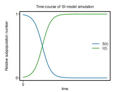
The susceptible population decreases with the conversion rate \(-\beta SI\), which depends on encounters between susceptible and infectious individuals and on the parameter \(\beta\), representing the strength or speed of change. The equation for the infectious population has the same rate with a positive sign. For the typical case in which almost 100% of individuals are susceptible at time 0, the temporal solutions for both groups follow a sigmoidal course (logistic function): an initial phase of exponential growth of the infectious group followed by saturation, where all formerly susceptible individuals eventually become infectious.

“SIS” model

A possible extension of the SI model assumes that infectious individuals can become susceptible again, which changes the differential equations as follows:

One interpretation of this SIS model is that infectious individuals mount an immune response that returns them to the susceptible group, but without developing permanent immunity, so reinfection remains possible. This happens with the “total recovery rate” \(bI\). An alternative interpretation is the simultaneous presence of a recovery rate \(\gamma I\), a birth rate \(\mu (N - S)\), which continuously adds new susceptible individuals, and a death rate among the infectious \(\mu I\), which exactly balances the birth rate.

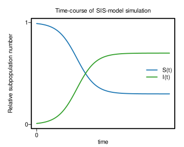
Compared with the SI model, the temporal dynamics of the two groups now approach an equilibrium that does not converge to 100% infectious and 0% susceptible individuals.

“SIR” model

An alternative extension of the SI model describes disease spread with permanent immunity. A third state variable \(R\) is introduced, representing individuals who can no longer become infected (with total population size \(N = S + I + R = \text{const.}\)):

The abbreviation \(R\) stands for “recovered” or “removed”. The latter is an interpretational choice and may reflect removal from the infectious group by immunity or by death. In the case of immunity, \(\gamma I\) is interpreted as the immunisation rate.

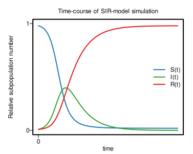
The temporal solution of the SIR model typically shows a rise in infectious individuals over a certain period, followed by a decline after a peak, while the susceptible group approaches 0% and the recovered group approaches 100% of the population.

“SIRS” model

In the SIRS model there are birth and death rates and, most importantly, immunity is assumed to be temporary: recovered individuals can become susceptible again via the rate \(fR\) after a characteristic time delay:

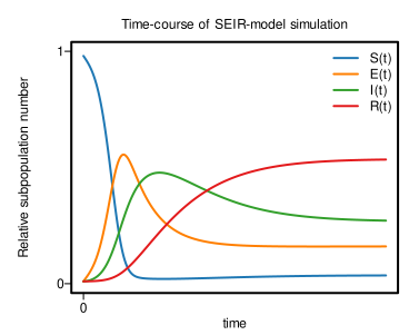
These effects lead, on the one hand, to characteristic temporal courses of all three variables and, on the other hand, to an equilibrium in which the groups settle at values between 0% and 100% of the total population, depending on the parameter set.

References

- [1] M. Niazi and A. Hussain: Agent-based computing from multi-agent systems to agent-based models: a visual survey. In: Scientometrics, 89:479–499, 2011. doi: 10.1007/s11192-011-0468-9
- [2] L. Perez and S. Dragicevic: An agent-based approach for modeling dynamics of contagious disease spread. In: Int. J. Health Geogr., 8:50, 2009. doi: 10.1186/1476-072X-8-50
- [3] W. O. Kermack and A. G. McKendrick: A contribution to the mathematical theory of epidemics. In: Proceedings of the Royal Society of London A, 115:700–721, 1927. doi: 10.1098/rspa.1927.0118