
With our model-based bioprocess optimisation, you can significantly increase the economic efficiency and productivity of your upstream processes. Using recombinant bioproduct manufacturing as an example, we use mathematical models to identify the exact levers for your success. By precisely computing optimal control variables – such as substrate concentration as well as the exact activation and harvest times – productivity can be increased by around 70% in practice. Our tailored approach maximises product concentration while reducing biomass accumulation, which substantially simplifies and accelerates downstream purification.
(Status: February 2022)
Application example
The genetically modified organism \(\color{#4daf4a}{X}\) (cf. E. coli) is cultivated in an ideally mixed stirred-tank reactor. Formation of the recombinant product \(\color{#377eb8}{P}\) is induced by adding an activator \(a\) (cf. IPTG) at time \(t_{\text{a}}\).[1] Biomass growth and product formation both compete for the same substrate \(\color{#ff7f00}{S}\) (cf. glucose). At the end of the process duration \(t_{\text{harvest}}\), the product is harvested and processed. The time courses of the state variables for the non-optimised bioprocess are shown in the figure below:
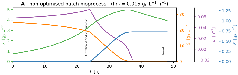
The figure shows that high substrate concentrations \(\color{#ff7f00}{S}\) inhibit biomass growth \(\color{#984ea3}{\mu}\). After addition of the activator, most of the substrate is consumed for product formation, and increasing product concentration further inhibits biomass growth. Once the substrate is depleted, product formation stagnates, and biomass decay becomes evident. The bioprocess productivity \(Pr_{\text{P}}\) is calculated at the end of the process as the ratio of the change in product concentration to the elapsed process time:
\[ Pr_{\text{P}} = \frac{P(t_{\text{harvest}})-P(t_{0})}{t_{\text{harvest}}-t_{0}} \]Furthermore, the model required for model-based optimisation is assumed to be known and can be expressed as a system of differential equations.[2][3] In this case, it is given by:
\[ \dot{X} = \mu(S,P)\,X - k_{\text{d}} X \] \[ \dot{S} = -\frac{\mu(S,P)\,X}{Y_{\text{X,S}}} -\frac{\rho(S,a)\,X}{Y_{\text{P,S}}} - m X \] \[ \dot{P} = \rho(S,a)\,X \]Here, \(k_{\text{d}}\) and \(m\) denote constant rates for biomass decay and substrate consumption for cellular maintenance. The yield coefficients \(Y_{\text{X,S}}\) and \(Y_{\text{P,S}}\) represent the ratios of consumed substrate to newly formed biomass and product. Biomass growth/decay and product formation are described by the following kinetic functions:[2]
\[ \mu(S,P) = \frac{\mu_{\max} S} {K_{\text{S}} + S + \frac{S^2}{K_{\text{I,S}}} + \frac{S P}{K_{\text{I,P}}}} \] \[ \rho(S,a) = \begin{cases} 0, & \text{for } a = 0 \\[4pt] \dfrac{\rho_{\max} S}{K_{\text{P}} + S}, & \text{for } a = 1 \end{cases} \]The table below lists the model parameters used in this example:
| Symbol | Description | Value | Unit |
|---|---|---|---|
| $\mu_{\max}$ | maximum specific growth rate | $0.32$ | $\text{h}^{-1}$ |
| $\rho_{\max}$ | maximum specific product formation rate | $0.020$ | $\text{h}^{-1}$ |
| $K_{\text{S}}$ | substrate half-saturation constant | $2.3$ | $\text{g}_{\text{S}} \cdot \text{L}^{-1}$ |
| $K_{\text{P}}$ | product half-saturation constant | $1.6$ | $\text{g}_{\text{S}} \cdot \text{L}^{-1}$ |
| $K_{\text{I,S}}$ | substrate inhibition constant | $9.1$ | $\text{g}_{\text{S}} \cdot \text{L}^{-1}$ |
| $K_{\text{I,P}}$ | product inhibition constant | $0.10$ | $\text{g}_{\text{P}} \cdot \text{L}^{-1}$ |
| $k_{\text{d}}$ | specific biomass decay rate | $0.024$ | $\text{h}^{-1}$ |
| $m$ | specific substrate maintenance rate | $0.034$ | $\text{g}_{\text{S}} \cdot \text{g}_{\text{X}}^{-1} \cdot \text{h}^{-1}$ |
| $Y_{\text{X,S}}$ | yield coefficient biomass/substrate | $0.60$ | $\text{g}_{\text{X}} \cdot \text{g}_{\text{S}}^{-1}$ |
| $Y_{\text{P,S}}$ | yield coefficient product/substrate | $0.053$ | $\text{g}_{\text{P}} \cdot \text{g}_{\text{S}}^{-1}$ |
Methodological background
In general, optimisation of a bioprocess means targeted manipulation of the operating mode of bioreactors with respect to one or more quantitative objectives. Typical objectives include minimisation of process time or energy, as well as of expensive or toxic substrates.[4] In this example, bioprocess productivity \(Pr_{\text{P}}\) is the sole objective.
It must also be possible to intervene in the process via suitable control variables. These are either known or can be identified using data analysis or simulations (e.g. sensitivity analysis). Furthermore, optimisation assumes the availability of a parametrised mathematical model of the process that is capable of capturing all essential process features. Here, the substrate concentration \(\color{#ff7f00}{S}\) at the start of cultivation \(t_{0}\), the activation time of product formation \(t_{\text{a}}\) and the harvest time \(t_{\text{harvest}}\) are defined as control variables.
Methodologically, model-based optimisation can be divided into two groups. First, computation of an optimal control profile for dynamic processes (“dynamic” optimisation), where time-varying control trajectories are sought. Second, determination of static values for the control variables, which in part resembles parameter identification. In both cases, control settings are determined that minimise or maximise the chosen objective. In this example, a static optimisation is used:
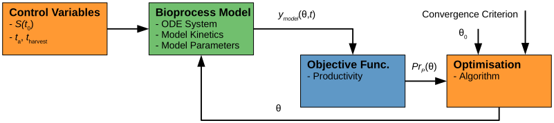
In the scheme above, the control variables \(S(t_{0})\), \(t_{\text{a}}\) and \(t_{\text{harvest}}\) are collected in the vector \(\theta\). The optimal control values \(\Omega\) are obtained by maximising the objective:
\[ \Omega = \underset{\theta}{\text{arg max}}\,Pr_{\text{P}}(\theta) \]Optimisation is implemented as mathematical minimisation/maximisation. Many established methods can be used, including deterministic approaches (e.g. gradient-based methods or simplex methods[5]) and heuristic approaches (e.g. genetic algorithms[6], simulated annealing), as well as hybrid combinations.
Both dynamic and static constraints on the control variables must be taken into account, typically expressed as systems of equalities and inequalities. In this example, these include \(S(t_{0}) \gt 0\), \(t_{\text{a}} \gt 0\) and \(t_{\text{harvest}} \gt 0\) (static) as well as \(t_{\text{a}} \lt t_{\text{harvest}}\) (dynamic).
Optimisation results
Comparing subfigure A (“non-optimised bioprocess”) with subfigure B (“optimised bioprocess”) in the figure below shows that the productivity objective \(Pr_{\text{P}}\) could be increased by approximately \(70\%\).
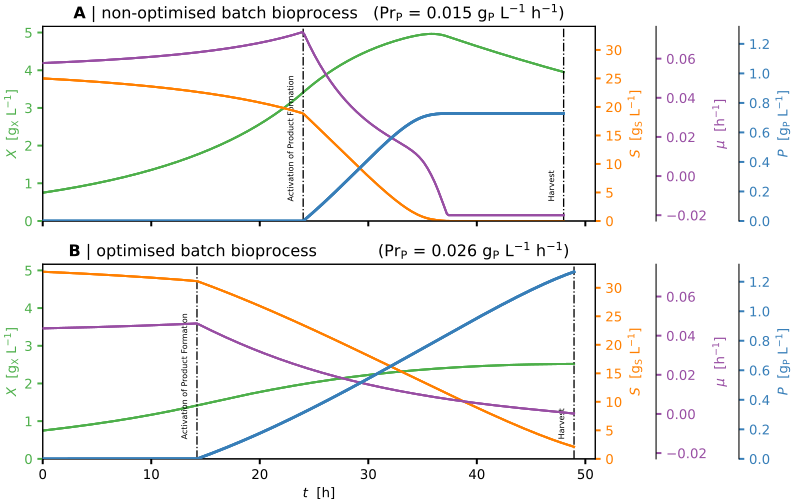
This improvement was achieved primarily by appropriately increasing the initial substrate concentration \(\color{#ff7f00}{S}\) and by extending the product formation phase (earlier addition of the activator \(a\)). The harvest time \(t_{\text{harvest}}\) was adjusted only slightly.
In addition to the increased productivity \(Pr_{\text{P}}\), the substantially higher absolute product concentration \(\color{#377eb8}{P}\) and reduced biomass accumulation \(\color{#4daf4a}{X}\) are noteworthy. Both effects are highly beneficial for the subsequent downstream processing of the culture. The table below lists the control variables used in this example and the resulting productivity; optimised values are shown in bold:
| Symbol | Description | Value non-optimised | Value optimised | Unit |
|---|---|---|---|---|
| $X_0$ | biomass concentration at start | $0.75$ | $0.75$ | $\text{g}_{\text{X}} \cdot \text{L}^{-1}$ |
| $S_0$ | substrate concentration at start | $25$ | $\mathbf{33}$ | $\text{g}_{\text{S}} \cdot \text{L}^{-1}$ |
| $P_0$ | product concentration at start | $0$ | $0$ | $\text{g}_{\text{P}} \cdot \text{L}^{-1}$ |
| $t_{\text{a}}$ | time of activation of product formation | $24$ | $\mathbf{14}$ | $\text{h}$ |
| $t_{\text{harvest}}$ | harvest time | $48$ | $\mathbf{49}$ | $\text{h}$ |
| $Pr_{\text{P}}$ | productivity | $0.015$ | $\mathbf{0.026}\text{ }(+73\,\%)$ | $\text{g}_{\text{P}} \cdot \text{L}^{-1} \cdot \text{h}^{-1}$ |
In this example, the initial biomass and product concentrations \(X_0\) and \(P_0\) were excluded from optimisation for simplicity. In real applications, however, all available control variables should be assessed for their sensitivity with respect to the objective and included in the optimisation strategy where appropriate.
Modifying the chosen bioprocess regime can also form part of the optimisation strategy, provided this is feasible technologically and economically. The present example considers a simple batch mode. Possible modifications include switching to fed-batch or repeated fed-batch operation, or to continuous modes (chemostat, turbidostat).[465] Where biotechnologically possible, immobilisation of biomass may also be considered as part of such modifications.
References
- [1] L. Gao, Y. Ren, Y. Ma, J. Lin and J. Lin: Modeling and simulation of production of metallothionein and red fluorescent fusion protein by recombinant Escherichia coli using graphical programming. In: Modeling, Programming and Simulations Using LabVIEW Software, IntechOpen, London, United Kingdom, 2011. doi: 10.5772/14091
- [2] D. Voet and J. G. Voet: Biochemistry. New York: John Wiley & Sons, 1990. ISBN: 0-471-61769-5
- [3] A. Kremling: Grundlagen der mathematischen Modellierung. In: Kompendium Systembiologie, Vieweg+Teubner Verlag, 2012. doi: 10.1007/978-3-8348-8607-1_3
- [4] J. A. Nelder and R. Mead: A simplex method for function minimization. In: The Computer Journal, 7(4):308–313, 1965. doi: 10.1093/comjnl/7.4.308
- [5] A. Raue et al.: Structural and practical identifiability analysis of partially observed dynamical models by exploiting the profile likelihood. In: Bioinformatics, 25(15):1923–1929, 2009. doi: 10.1093/bioinformatics/btp358
- [6] B. Tang: Orthogonal array-based latin hypercubes. In: Journal of the American Statistical Association, 88(424):1392–1397, 1993. doi: 10.2307/2291282
- [7] I. M. Sobol: Distribution of points in a cube and approximate evaluation of integrals. In: Zh. Vych. Mat. Mat. Fiz., 7:784–802, 1967.
- [8] A. Saltelli: Making best use of model evaluations to compute sensitivity indices. In: Computer Physics Communications, 145:280–297, 2002. doi: 10.1016/S0010-4655(02)00280-1